40 pie chart excel labels
Pie of Pie Chart in Excel - Inserting, Customizing, Formatting Inserting a Pie of Pie Chart. Let us say we have the sales of different items of a bakery. Below is the data:-. To insert a Pie of Pie chart:-. Select the data range A1:B7. Enter in the Insert Tab. Select the Pie button, in the charts group. Select Pie of Pie chart in the 2D chart section. Edit titles or data labels in a chart - support.microsoft.com On a chart, click the label that you want to link to a corresponding worksheet cell. On the worksheet, click in the formula bar, and then type an equal sign (=). Select the worksheet cell that contains the data or text that you want to display in your chart. You can also type the reference to the worksheet cell in the formula bar.
excel - How to not display labels in pie chart that are 0% - Stack Overflow Generate a new column with the following formula: =IF (B2=0,"",A2) Then right click on the labels and choose "Format Data Labels". Check "Value From Cells", choosing the column with the formula and percentage of the Label Options. Under Label Options -> Number -> Category, choose "Custom". Under Format Code, enter the following:

Pie chart excel labels
Everything You Need to Know About Pie Chart in Excel How to Make a Pie Chart in Excel Start with selecting your data in Excel. If you include data labels in your selection, Excel will automatically assign them to each column and generate the chart. Go to the INSERT tab in the Ribbon and click on the Pie Chart icon to see the pie chart types. Click on the desired chart to insert. How to Create and Label a Pie Chart in Excel 2013 Step 8: Label the Chart. Check the "Data Labels" square and the labels will appear on the pie chart. Congratulations, you have successfully created a labeled pie chart. Note: If you want to re-position the labels, hover your cursor over the "Data Labels" option and click on the small, black triangle that appears next to it. How to Insert Axis Labels In An Excel Chart | Excelchat Figure 2 - Adding Excel axis labels. Next, we will click on the chart to turn on the Chart Design tab. We will go to Chart Design and select Add Chart Element. Figure 3 - How to label axes in Excel. In the drop-down menu, we will click on Axis Titles, and subsequently, select Primary Horizontal. Figure 4 - How to add excel horizontal axis ...
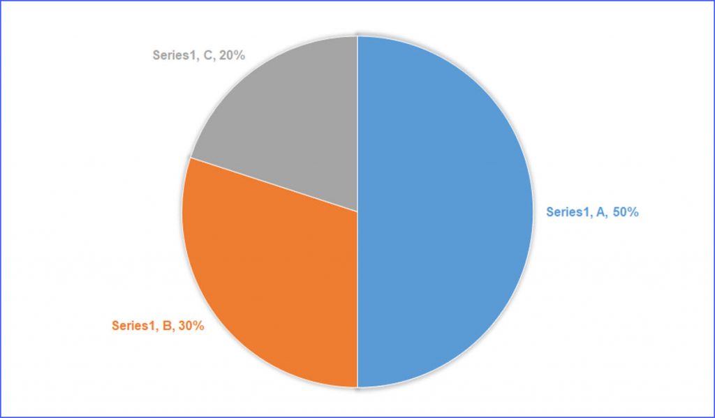
Pie chart excel labels. How to Create Pie Charts in Excel (In Easy Steps) Select the pie chart. 9. Click the + button on the right side of the chart and click the check box next to Data Labels. 10. Click the paintbrush icon on the right side of the chart and change the color scheme of the pie chart. Result: 11. Right click the pie chart and click Format Data Labels. 12. Pie Chart in Excel | How to Create Pie Chart | Step-by-Step ... Pie Chart in Excel is used for showing the completion or main contribution of different segments out of 100%. It is like each value represents the portion of the Slice from the total complete Pie. For Example, we have 4 values A, B, C and D. Creating Pie Chart and Adding/Formatting Data Labels (Excel) Creating Pie Chart and Adding/Formatting Data Labels (Excel) How to add axis label to chart in Excel? - ExtendOffice 1. Select the chart that you want to add axis label. 2. Navigate to Chart Tools Layout tab, and then click Axis Titles, see screenshot: 3. You can insert the horizontal axis label by clicking Primary Horizontal Axis Title under the Axis Title drop down, then click Title Below Axis, and a text box will appear at the bottom of the chart, then you ...
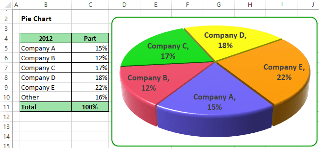
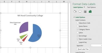
How to Use Cell Values for Excel Chart Labels Select the chart, choose the "Chart Elements" option, click the "Data Labels" arrow, and then "More Options.". Uncheck the "Value" box and check the "Value From Cells" box. Select cells C2:C6 to use for the data label range and then click the "OK" button. The values from these cells are now used for the chart data labels. Add or remove data labels in a chart - support.microsoft.com Click the data series or chart. To label one data point, after clicking the series, click that data point. In the upper right corner, next to the chart, click Add Chart Element > Data Labels. To change the location, click the arrow, and choose an option. If you want to show your data label inside a text bubble shape, click Data Callout. Microsoft Excel Tutorials: Add Data Labels to a Pie Chart You should get the following menu: From the menu, select Add Data Labels. New data labels will then appear on your chart: The values are in percentages in Excel 2007, however. To change this, right click your chart again. From the menu, select Format Data Labels: When you click Format Data Labels , you should get a dialogue box. How to Create a Pie Chart in Excel | Smartsheet To create a pie chart in Excel 2016, add your data set to a worksheet and highlight it. Then click the Insert tab, and click the dropdown menu next to the image of a pie chart. Select the chart type you want to use and the chosen chart will appear on the worksheet with the data you selected.
Pie Chart Best Fit Labels Overlapping - VBA Fix - Microsoft Tech Community I created attached Pie chart in Excel with 31 points and all labels are readable and perfectly placed. It is created from few clicks without VBA using data visualization tool in Excel. Data Visualization Tool For Excel Data Visualization Tool For Google Sheets It has auto cluttering effect to adjust according to your data size. How to Create and Format a Pie Chart in Excel - Lifewire Jan 23, 2021 · Select the plot area of the pie chart. Right-click the chart. Select Add Data Labels . Select Add Data Labels. In this example, the sales for each cookie is added to the slices of the pie chart. Change Colors When a chart is created in Excel, or whenever an existing chart is selected, two additional tabs are added to the ribbon. Chart Legend / Data Labels In Pie Chart | MrExcel Message Board Add the data labels. Then, right click on any data label to select all the data labels for that series and select Format Data Labels... From the Label Options tab, in the Label Contains section, select the 'Series Name' checkbox. The above applies to Excel 2007. Excel 2003 supports the same capability though the dialog box choices may be different. How to fix wrapped data labels in a pie chart - Sage Intelligence Right click on the data label and select Format Data Labels. 2. Select Text Options > Text Box > and un-select Wrap text in shape. 3. The data labels resize to fit all the text on one line. 4. Alternatively, by double-clicking a data label, the handles can be used to resize the label to wrap words as desired. This can be done on all data labels ...
31 How To Label Pie Charts In Excel - Labels Database 2020
How to display leader lines in pie chart in Excel? - ExtendOffice To display leader lines in pie chart, you just need to check an option then drag the labels out. 1. Click at the chart, and right click to select Format Data Labels from context menu. 2. In the popping Format Data Labels dialog/pane, check Show Leader Lines in the Label Options section. See screenshot: 3.
How to Make Labels the Same Color as the Pies in Pie Chart - ExcelNotes
Inserting Data Label in the Color Legend of a pie chart Hi, I am trying to insert data labels (percentages) as part of the side colored legend, rather than on the pie chart itself, as displayed on the image ... Microsoft Excel; Excel; Inserting Data Label in the Color Legend of a pie chart; Inserting Data Label in the Color Legend of a pie chart. Discussion Options. Subscribe to RSS Feed;

How to make a pie chart in Excel
How to Make a PIE Chart in Excel (Easy Step-by-Step Guide) Here are the steps to format the data label from the Design tab: Select the chart. This will make the Design tab available in the ribbon. In the Design tab, click on the Add Chart Element (it's in the Chart Layouts group). Hover the cursor on the Data Labels option.
Excel 3-D Pie Charts - Microsoft Excel 2013
Excel custom pie chart labels - Microsoft Community Excel custom pie chart labels I have a data set like this (basically form output): I want to use a pivot table to make a pie chart out of this. I want each of the pieces of the pie to contain the number of entries and between parentheses the percentage. So in the "Yes" piece, there should be '3 (33%)'.

How to make a pie chart in Excel
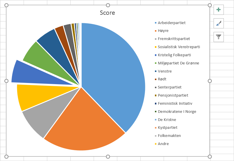
Only Display Some Labels On Pie Chart - Excel Help Forum Only Display Some Labels On Pie Chart. I have a pie chart that contains over 50 categories (Yes, I know pie charts shouldn't be used for that many things) but I want to only display labels for maybe the top 5 values or any label with a value >10. This is because there are a few standout values but I want all the other values to remain in the ...
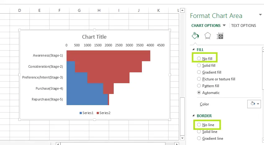
Funnel Chart in Excel - DataScience Made Simple
excel - Positioning data labels in pie chart - Stack Overflow Positioning data labels in pie chart. I'm trying to format some charts I have, using VBA. To get started I recorded a macro of me doing what I wanted, to have an idea of what methods I'd want etc. The recorded macro looks like this - I'm including the whole thing, though the line to pay attention to is Selection.Position = xlLabelPositionCenter.

How to Make a Pie Chart in Excel & Add Rich Data Labels to The Chart!
Pie Chart in Excel – Inserting, Formatting, Filters, Data Labels Dec 29, 2021 · Right click on the Data Labels on the chart. Click on Format Data Labels option. Consequently, this will open up the Format Data Labels pane on the right of the excel worksheet. Mark the Category Name, Percentage and Legend Key. Also mark the labels position at Outside End. This is how the chark looks. Formatting the Chart Background, Chart Styles
4.1 Choosing a Chart Type – Beginning Excel
How to Rotate Pie Chart in Excel? - WallStreetMojo Move the cursor to the chart area to select the pie chart. Step 5: Click on the Pie chart and select the 3D chart, as shown in the figure, and develop a 3D pie chart. Step 6: In the next step, change the title of the chart and add data labels to it. Step 7: To rotate the pie chart, click on the chart area.

33 How To Label Pie Chart In Excel - Labels Design Ideas 2020
Pie Chart Labels - Excel Help Forum I recently discovered a curious "feature" of Excel. If you create a pie chart, and label the slices of the pie with data labels that include the percentage, Excel sometimes adjusts the values in unexpected ways. As far as I can tell, this only happens when the percentages are formatted as whole-number percents (e.g., "57%"). In this situation, Excel will adjust values so that the sum of all of ...

Pie Chart – Excel Tutorials
Formatting data labels and printing pie charts on Excel for Mac 2019 ... Here's a work around I found for printing pie charts. Still can't find a solution for formatting the data labels. 1. When printing a pie chart from Excel for mac 2019, MS instructions are to select the chart only, on the worksheet > file > print. Excel is supposed to print the chart only (not the data ) and automatically fit it onto one page.

How to Create a Pie Chart in Microsoft Excel
How to Insert Axis Labels In An Excel Chart | Excelchat Figure 2 - Adding Excel axis labels. Next, we will click on the chart to turn on the Chart Design tab. We will go to Chart Design and select Add Chart Element. Figure 3 - How to label axes in Excel. In the drop-down menu, we will click on Axis Titles, and subsequently, select Primary Horizontal. Figure 4 - How to add excel horizontal axis ...
Pie Chart without Labels - Automate Excel
How to Create and Label a Pie Chart in Excel 2013 Step 8: Label the Chart. Check the "Data Labels" square and the labels will appear on the pie chart. Congratulations, you have successfully created a labeled pie chart. Note: If you want to re-position the labels, hover your cursor over the "Data Labels" option and click on the small, black triangle that appears next to it.
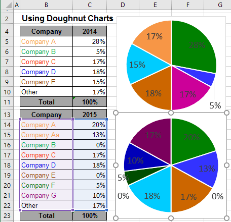
Using Pie Charts and Doughnut Charts in Excel
Everything You Need to Know About Pie Chart in Excel How to Make a Pie Chart in Excel Start with selecting your data in Excel. If you include data labels in your selection, Excel will automatically assign them to each column and generate the chart. Go to the INSERT tab in the Ribbon and click on the Pie Chart icon to see the pie chart types. Click on the desired chart to insert.
13. Extract a slice from the pie – bioST@TS
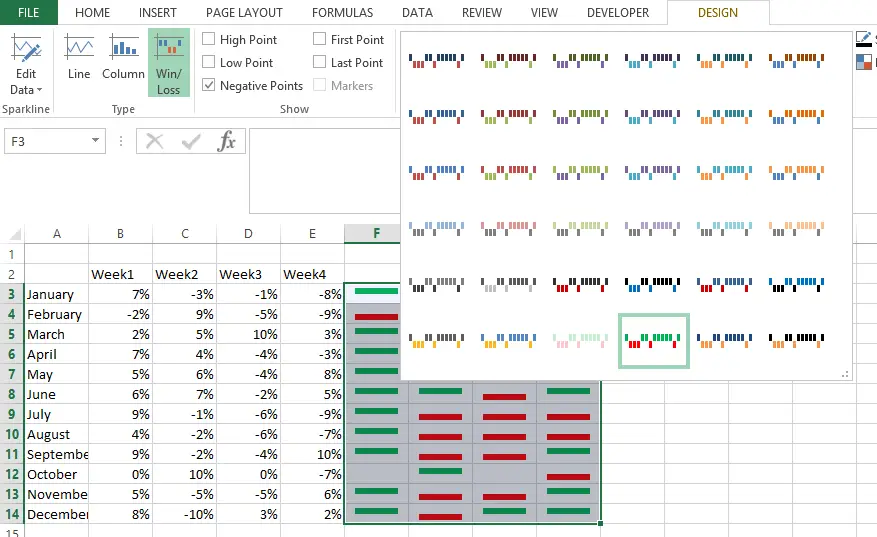
Win Loss Chart in Excel - DataScience Made Simple
Create a Pie Chart in Excel - Easy Excel Tutorial
Post a Comment for "40 pie chart excel labels"