42 excel scatter chart with labels
Scatter chart horizontal axis labels | MrExcel Message Board If you must use a XY Chart, you will have to simulate the effect. Add a dummy series which will have all y values as zero. Then, add data labels for this new series with the desired labels. Locate the data labels below the data points, hide the default x axis labels, and format the dummy series to have no line and no marker. oereich said: Hi, Create an X Y Scatter Chart with Data Labels - YouTube How to create an X Y Scatter Chart with Data Label. There isn't a function to do it explicitly in Excel, but it can be done with a macro. The Microsoft Kno...
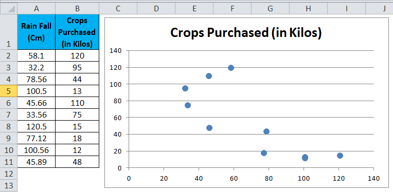
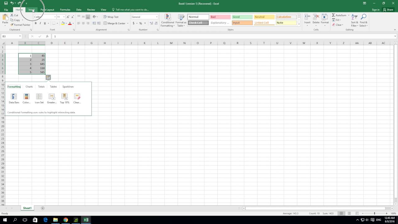
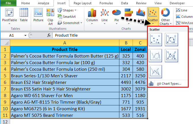
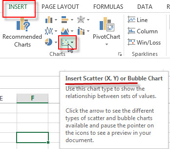
How To Create Scatter Chart in Excel? - EDUCBA To apply the scatter chart by using the above figure, follow the below-mentioned steps as follows. Step 1 - First, select the X and Y columns as shown below. Step 2 - Go to the Insert menu and select the Scatter Chart. Step 3 - Click on the down arrow so that we will get the list of scatter chart list which is shown below.
Excel scatter chart with labels
Scatter Plots in Excel with Data Labels Select "Chart Design" from the ribbon then "Add Chart Element" Then "Data Labels". We then need to Select again and choose "More Data Label Options" i.e. the last option in the menu. This will... Creating Scatter Plot with Marker Labels - Microsoft Community Right click any data point and click 'Add data labels and Excel will pick one of the columns you used to create the chart. Right click one of these data labels and click 'Format data labels' and in the context menu that pops up select 'Value from cells' and select the column of names and click OK. Scatter Plot with Text Labels on X-axis : excel For example, consider a formula like this: =IF (XLOOKUP (A1,B:B,C:C)>5,XLOOKUP (A1,B:B,C:C)+3,XLOOKUP (A1,B:B,C:C)-2) So basically a lookup or something else with a bit of complexity, is referenced multiple times. Now this isn't too bad in this example, but you can often have instances where you need to call the same sub-function multiple times ...
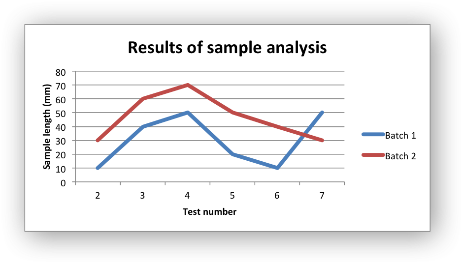
Excel scatter chart with labels. Multiple Time Series in an Excel Chart - Peltier Tech Aug 12, 2016 · Any of the formatting described here applies to all of these chart types. XY Scatter charts are different: X axes behave like Y axes. I could write a book just on this subject. Displaying Multiple Time Series in An Excel Chart. The usual problem here is that data comes from different places. How to use a macro to add labels to data points in an xy ... The labels and values must be laid out in exactly the format described in this article. (The upper-left cell does not have to be cell A1.) To attach text labels to data points in an xy (scatter) chart, follow these steps: On the worksheet that contains the sample data, select the cell range B1:C6. What is a 3D Scatter Plot Chart in Excel? - projectcubicle Select the data set that you want to plot on the chart. 2. Go to Insert tab > Charts group > select Scatter chart from the drop-down menu or click on the Insert button from Charts group, then select Scatter chart from the Insert dialog box. 3. How to Create a Quadrant Chart in Excel - Automate Excel Click the " Insert Scatter (X, Y) or Bubble Chart. " Choose " Scatter. " Step #2: Add the values to the chart. Once the empty chart appears, add the values from the table with your actual data. Right-click on the chart area and choose " Select Data ." Another menu will come up. Under Legend Entries (Series), click the " Add " button.
How to find, highlight and label a data point in Excel scatter plot Select the Data Labels box and choose where to position the label. By default, Excel shows one numeric value for the label, y value in our case. To display both x and y values, right-click the label, click Format Data Labels…, select the X Value and Y value boxes, and set the Separator of your choosing: Label the data point by name How to add axis label to chart in Excel? - ExtendOffice 1. Select the chart that you want to add axis label. 2. Navigate to Chart Tools Layout tab, and then click Axis Titles, see screenshot: 3. You can insert the horizontal axis label by clicking Primary Horizontal Axis Title under the Axis Title drop down, then click Title Below Axis, and a text box will appear at the bottom of the chart, then you ... How to display text labels in the X-axis of scatter chart in ... Display text labels in X-axis of scatter chart. Actually, there is no way that can display text labels in the X-axis of scatter chart in Excel, but we can create a line chart and make it look like a scatter chart. 1. Select the data you use, and click Insert > Insert Line & Area Chart > Line with Markers to select a line chart. See screenshot: scatter-plot-with-labels | Real Statistics Using Excel scatter-plot-with-labels. Leave a Comment Cancel reply. Comment. Name Email Website. ... Excel Capabilities; Matrices and Iterative Procedures; Linear Algebra and Advanced Matrix Topics; Other Mathematical Topics; Statistics Tables; Bibliography; Author; Citation; Blogs; Tools. Distribution Functions;
Add or remove data labels in a chart - support.microsoft.com Click the data series or chart. To label one data point, after clicking the series, click that data point. In the upper right corner, next to the chart, click Add Chart Element > Data Labels. To change the location, click the arrow, and choose an option. If you want to show your data label inside a text bubble shape, click Data Callout. How to Add Labels to Scatterplot Points in Excel - Statology Step 3: Add Labels to Points. Next, click anywhere on the chart until a green plus (+) sign appears in the top right corner. Then click Data Labels, then click More Options…. In the Format Data Labels window that appears on the right of the screen, uncheck the box next to Y Value and check the box next to Value From Cells. How to Find, Highlight, and Label a Data Point in Excel Scatter Plot? By default, the data labels are the y-coordinates. Step 3: Right-click on any of the data labels. A drop-down appears. Click on the Format Data Labels… option. Step 4: Format Data Labels dialogue box appears. Under the Label Options, check the box Value from Cells . Step 5: Data Label Range dialogue-box appears. Excel Chart Vertical Axis Text Labels - My Online Training Hub So all we need to do is get that bar chart into our line chart, align the labels to the line chart and then hide the bars. We’ll do this with a dummy series: Copy cells G4:H10 (note row 5 is intentionally blank) > CTRL+C to copy the cells > select the chart > CTRL+V to paste the dummy data into the chart.
Scatter Chart in Excel (Uses, Examples) | How To Create Scatter Chart?
Add Custom Labels to x-y Scatter plot in Excel Step 1: Select the Data, INSERT -> Recommended Charts -> Scatter chart (3 rd chart will be scatter chart) Let the plotted scatter chart be. Step 2: Click the + symbol and add data labels by clicking it as shown below. Step 3: Now we need to add the flavor names to the label. Now right click on the label and click format data labels.
Example: Line Chart — XlsxWriter Documentation
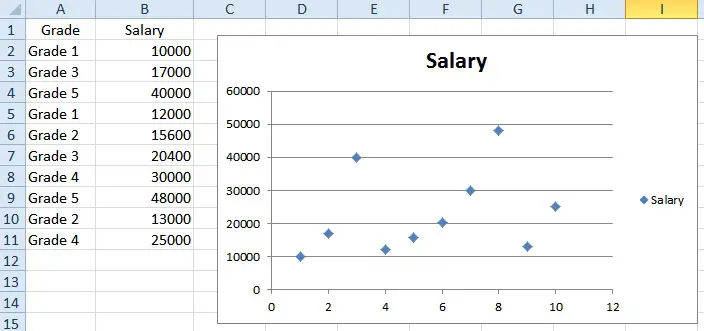
Excel scatter chart using text name - Access-Excel.Tips Since Excel allows different chart types to be displayed in one chart, we are going to create a mix of bar chart (column chart) and scatter chart. Scatter chart is used to display the actual data point, while bar chart is to display Grade labels. - Create scatter chart for Range B20:C31 (Series 1)
Excel scatter chart using text name - Access-Excel.Tips
Excel Scatter Chart with Labels - Super User Move the button down and out of the way of your data if you have more than a few columns. Paste your data in on top of the film data. Create scatter plots by selecting two column at a time and insert scatter (plot). Clicking on the button, which will add labels. Easy.
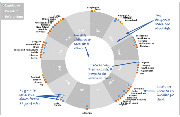
Combine pie and xy scatter charts - Advanced Excel Charting Example
Excel: labels on a scatter chart, read from array - Stack Overflow Excel: labels on a scatter chart, read from array Ask Question 0 Here I have a chart I did a right-click -> "Add labels" , and it read them from my a (H/C) row. Basically, I want it to read label values from the CO2/CH4 row instead, so they would be 0,0.5,1,2,5,10 instead.
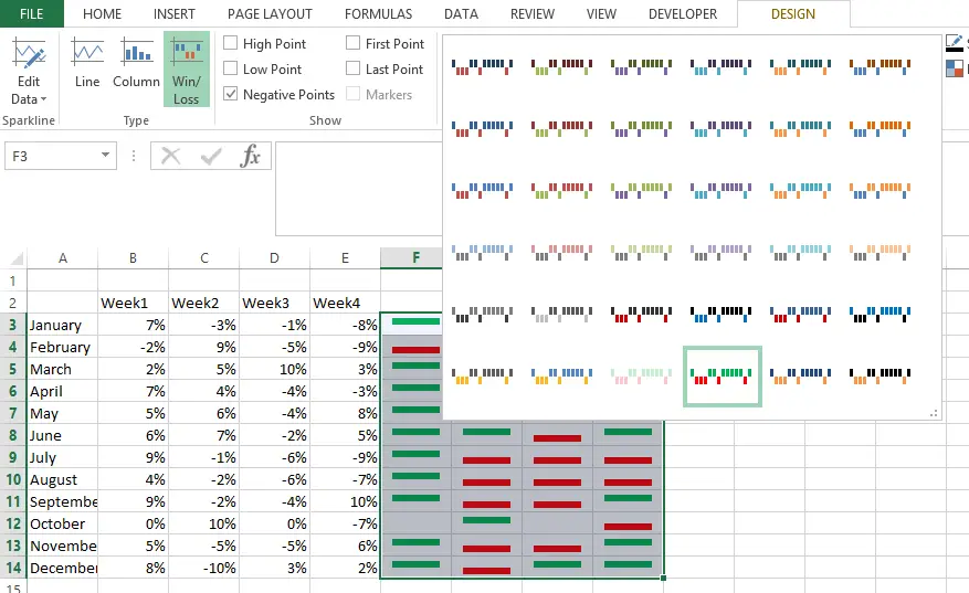
Win Loss Chart in Excel - DataScience Made Simple
Add vertical line to Excel chart: scatter plot, bar and line ... May 15, 2019 · In Excel 2013, Excel 2016, Excel 2019 and later, select Combo on the All Charts tab, choose Scatter with Straight Lines for the Average series, and click OK to close the dialog. In Excel 2010 and earlier, select X Y (Scatter) > Scatter with Straight Lines , and click OK .

Scatter Chart in Microsoft Excel
How to Change Excel Chart Data Labels to Custom Values? May 05, 2010 · The Chart I have created (type thin line with tick markers) WILL NOT display x axis labels associated with more than 150 rows of data. (Noting 150/4=~ 38 labels initially chart ok, out of 1050/4=~ 263 total months labels in column A.) It does chart all 1050 rows of data values in Y at all times.

How to Add a Third Y-Axis to a Scatter Chart | EngineerExcel
Custom Axis Labels and Gridlines in an Excel Chart Jul 23, 2013 · Select the vertical dummy series and add data labels, as follows. In Excel 2007-2010, go to the Chart Tools > Layout tab > Data Labels > More Data label Options. In Excel 2013, click the “+” icon to the top right of the chart, click the right arrow next to Data Labels, and choose More Options….

Line Chart in Excel - Easy Excel Tutorial
How To Add Axis Labels In Excel [Step-By-Step Tutorial] First off, you have to click the chart and click the plus (+) icon on the upper-right side. Then, check the tickbox for 'Axis Titles'. If you would only like to add a title/label for one axis (horizontal or vertical), click the right arrow beside 'Axis Titles' and select which axis you would like to add a title/label.
How to create a scatter Chart in excel 2016 - YouTube
How do I set labels for each point of a scatter chart? Answer trip_to_tokyo Volunteer Moderator | Article Author Replied on September 14, 2011 Click one of the data points on the chart. Chart Tools. Layout contextual tab. Labels group. Click on the drop down arrow to the right of:- Data Labels Make your choice. If my comments have helped please vote as helpful. Thanks. Report abuse

Scatter Chart in Microsoft Excel
Labeling X-Y Scatter Plots (Microsoft Excel) Just enter "Age" (including the quotation marks) for the Custom format for the cell. Then format the chart to display the label for X or Y value. When you do this, the X-axis values of the chart will probably all changed to whatever the format name is (i.e., Age). However, after formatting the X-axis to Number (with no digits after the decimal ...

Excel: labels on a scatter chart, read from array - Stack Overflow
Improve your X Y Scatter Chart with custom data labels Select the x y scatter chart. Press Alt+F8 to view a list of macros available. Select "AddDataLabels". Press with left mouse button on "Run" button. Select the custom data labels you want to assign to your chart. Make sure you select as many cells as there are data points in your chart. Press with left mouse button on OK button. Back to top
Scatter Chart in Excel (Examples) | How To Create Scatter Chart in Excel?
Change hover label data on Scatter plot chart - MrExcel Message Board This means that I cant use ordinary labels, because it destroys all visibility of the chart. So I need to hover the dots to see the label data. This works good but I cant manage to get the names of the items on the hovering label. When I choose the data I can pick X data, Y data and series name. But when I choose a range for "series name" it ...
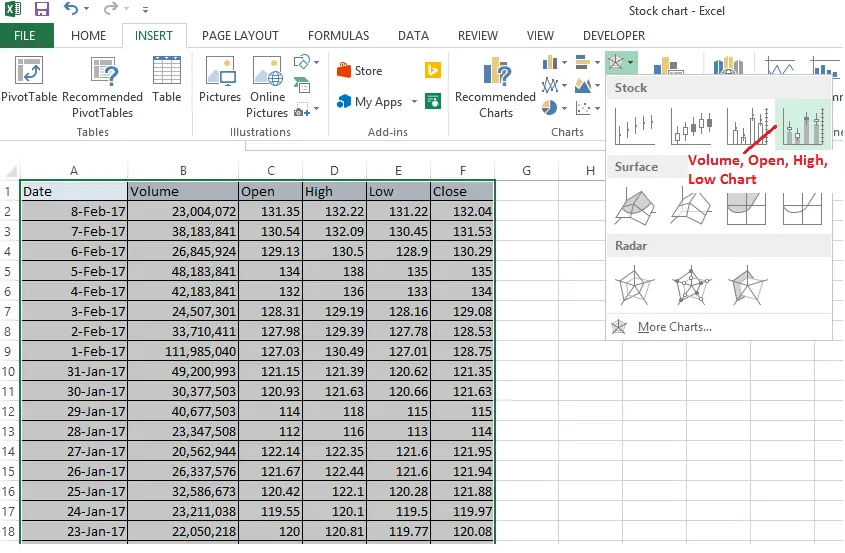
Stock chart in Excel or candlestick chart in Excel - DataScience Made Simple
excel - How to getting text labels to show up in scatter chart - Stack ... How to getting text labels to show up in scatter chart. I want text labels for my scatter plot that is connected with points in the graph. my data is like this. The chart removes the labels and places numbers. How do I get the text labels back?
Excel scatter Chart - Free Excel Tutorial
Hover labels on scatterplot points - Excel Help Forum You can not edit the content of chart hover labels. The information they show is directly related to the underlying chart data, series name/Point/x/y You can use code to capture events of the chart and display your own information via a textbox. Cheers Andy Register To Reply
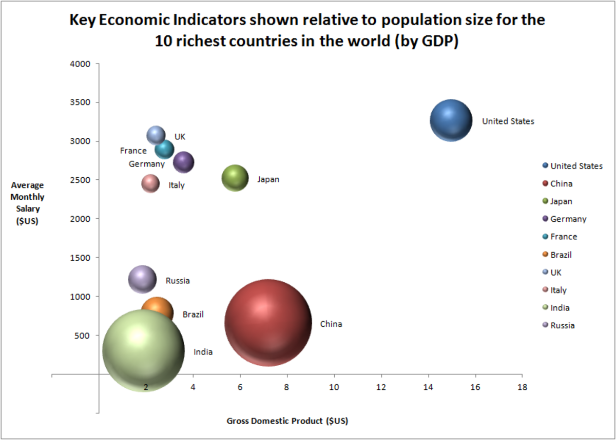
How to create and configure a bubble chart template in Excel 2007 and Excel 2010 | hubpages
how to make a scatter plot in Excel - storytelling with data Select "Scatter" from the options in the "Recommended Charts" section of your ribbon. Excel will automatically create a scatter plot for you in the same sheet as your data, using the first column of your dataset as the horizontal (X) axis, and the second column as your vertical (Y) axis. A quick note here: in creating scatter plots, a ...

Excel Charts | Real Statistics Using Excel
Scatter Plot with Text Labels on X-axis : excel For example, consider a formula like this: =IF (XLOOKUP (A1,B:B,C:C)>5,XLOOKUP (A1,B:B,C:C)+3,XLOOKUP (A1,B:B,C:C)-2) So basically a lookup or something else with a bit of complexity, is referenced multiple times. Now this isn't too bad in this example, but you can often have instances where you need to call the same sub-function multiple times ...
Post a Comment for "42 excel scatter chart with labels"