45 excel 2013 data labels

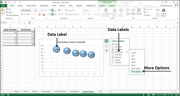
Excel Data Analysis - Data Visualization - tutorialspoint.com Data Labels. Excel 2013 and later versions provide you with various options to display Data Labels. You can choose one Data Label, format it as you like, and then use Clone Current Label to copy the formatting to the rest of the Data Labels in the chart. The Data Labels in a chart can have effects, varying shapes and sizes. Tutorial: Import Data into Excel, and Create a Data Model In the next tutorial, Extend Data Model relationships using Excel 2013, Power Pivot, and DAX, you build on what you learned here, and step through extending the Data Model using a powerful and visual Excel add-in called Power Pivot. You also learn how to calculate columns in a table, and use that calculated column so that an otherwise unrelated ...

What's new in Excel 2013 - support.microsoft.com Data labels stay in place, even when you switch to a different type of chart. You can also connect them to their data points with leader lines on all charts, not just pie charts. To work with rich data labels, see Change the format of data labels in a chart. View animation in charts. See a chart come alive when you make changes to its source data.

Excel 2013 data labels

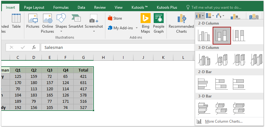
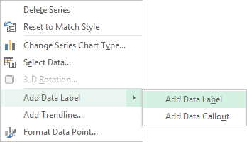
How to Add Total Data Labels to the Excel Stacked Bar Chart Apr 03, 2013 · Step 4: Right click your new line chart and select “Add Data Labels” Step 5: Right click your new data labels and format them so that their label position is “Above”; also make the labels bold and increase the font size. Step 6: Right click the line, select “Format Data Series”; in the Line Color menu, select “No line” Format Data Labels in Excel- Instructions - TeachUcomp, Inc. Nov 14, 2019 · Then select the “Format Data Labels…” command from the pop-up menu that appears to format data labels in Excel. Using either method then displays the “Format Data Labels” task pane at the right side of the screen. Format Data Labels in Excel- Instructions: A picture of the “Format Data Labels” task pane in Excel. Pivot table - Wikipedia For example, in Microsoft Excel one must first select the entire data in the original table and then go to the Insert tab and select "Pivot Table" (or "Pivot Chart"). The user then has the option of either inserting the pivot table into an existing sheet or creating a new sheet to house the pivot table.

Excel 2013 data labels. Excel Barcode Generator Add-in: Create Barcodes in Excel 2019 ... Office Excel Barcode Encoder Add-In is a reliable, efficient and convenient barcode generator for Microsoft Excel 2016/2013/2010/2007, which is designed for office users to embed most popular barcodes into Excel workbooks. It is widely applied in many industries. Pivot table - Wikipedia For example, in Microsoft Excel one must first select the entire data in the original table and then go to the Insert tab and select "Pivot Table" (or "Pivot Chart"). The user then has the option of either inserting the pivot table into an existing sheet or creating a new sheet to house the pivot table. Format Data Labels in Excel- Instructions - TeachUcomp, Inc. Nov 14, 2019 · Then select the “Format Data Labels…” command from the pop-up menu that appears to format data labels in Excel. Using either method then displays the “Format Data Labels” task pane at the right side of the screen. Format Data Labels in Excel- Instructions: A picture of the “Format Data Labels” task pane in Excel. How to Add Total Data Labels to the Excel Stacked Bar Chart Apr 03, 2013 · Step 4: Right click your new line chart and select “Add Data Labels” Step 5: Right click your new data labels and format them so that their label position is “Above”; also make the labels bold and increase the font size. Step 6: Right click the line, select “Format Data Series”; in the Line Color menu, select “No line”

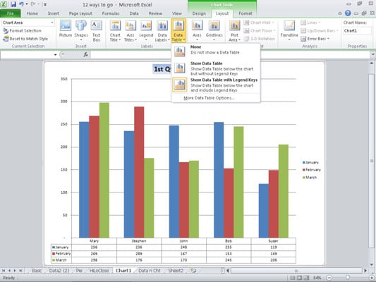
How to Add a Data Table to an Excel 2010 Chart - dummies

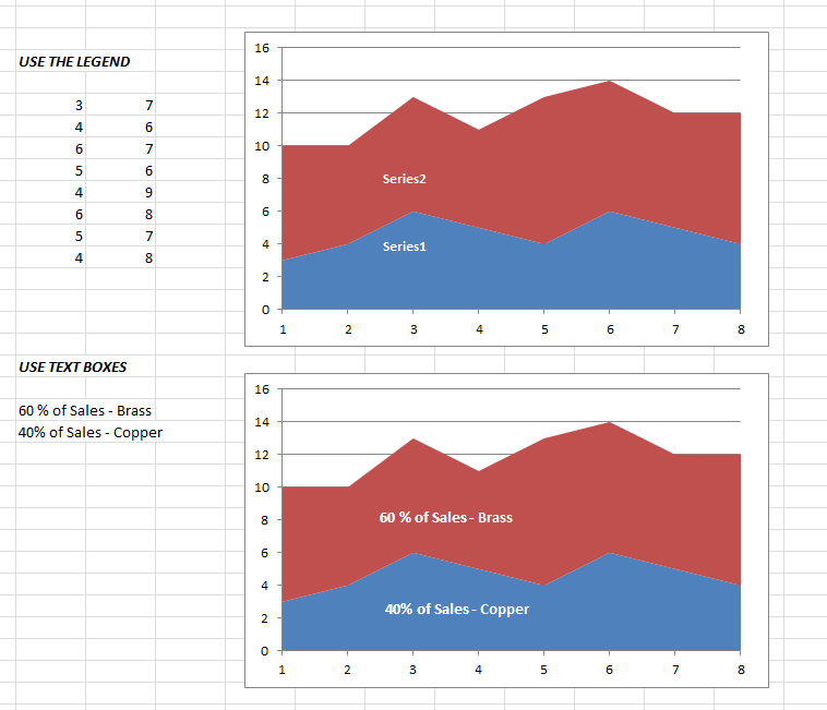
Area Chart Data Label | MrExcel Message Board

Custom data labels in a chart

Excel Tips n Tricks -Tip 8 (Applying Chart Data Labels From a ...

Custom Chart Labels Using Excel 2013 | MyExcelOnline

How to add total labels to stacked column chart in Excel?

How to Add Total Data Labels to the Excel Stacked Bar Chart ...

Custom Chart Labels Using Excel 2013 | MyExcelOnline

How To Show Or Hide Data Labels On MS Excel? | My Windows Hub

Add or remove data labels in a chart

Improve your X Y Scatter Chart with custom data labels

Directly Labeling Excel Charts - PolicyViz

Adding rich data labels to charts in Excel 2013 | Microsoft ...

Excel: Clustered Column Chart with Percent of Month ...

Add or remove data labels in a chart

Custom Data Labels with Colors and Symbols in Excel Charts ...

Directly Labeling in Excel

Microsoft Excel Tutorials: Add Data Labels to a Pie Chart

Adding a Benchmark Line to a Graph

Excel Charts - Aesthetic Data Labels

Excel charts: add title, customize chart axis, legend and ...

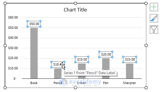
Fixed:] Excel Chart Is Not Showing All Data Labels (2 Solutions)

Add or remove data labels in a chart

How to add or move data labels in Excel chart?

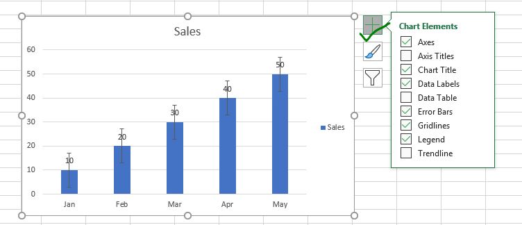
How to Add and Remove Chart Elements in Excel

Creating a chart with dynamic labels - Microsoft Excel 2013

How to Move Data Labels In Excel Chart (2 Easy Methods)

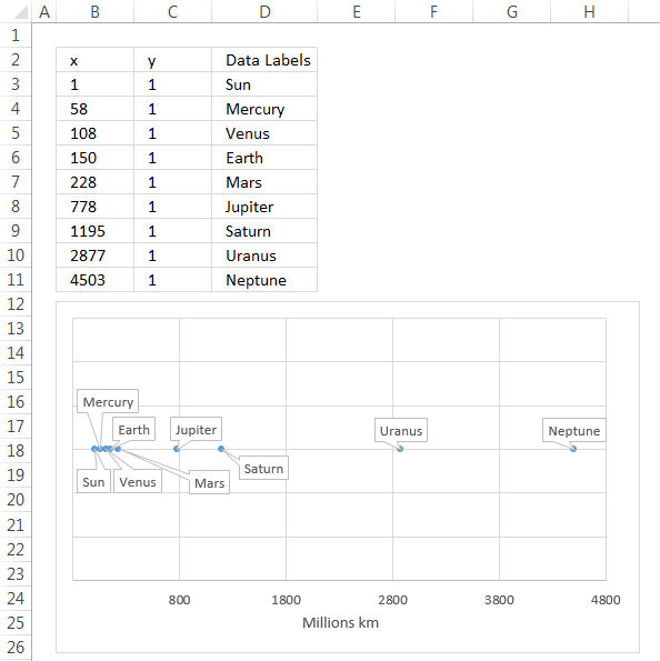
Improve your X Y Scatter Chart with custom data labels

Office: Display Data Labels in a Pie Chart

Excel Charts - Category Text

How to Make a Pie Chart in Excel – Contextures Blog

Custom data labels in a chart

Apply Custom Data Labels to Charted Points - Peltier Tech

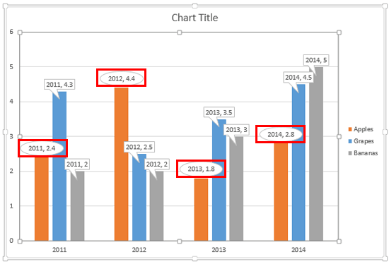
Change Callout Shapes for Data Labels in PowerPoint 2013 for ...

Creating Pie Chart and Adding/Formatting Data Labels (Excel)

Improve your X Y Scatter Chart with custom data labels

Directly Labeling Excel Charts - PolicyViz

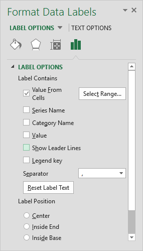
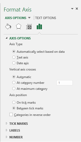
Change the format of data labels in a chart

Custom Excel Chart Label Positions • My Online Training Hub

Change the format of data labels in a chart

Apply Custom Data Labels to Charted Points - Peltier Tech

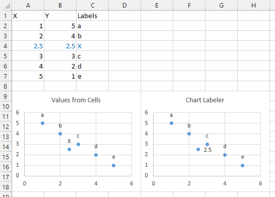
perl - Excel::Writer::XLSX - Data Label "Value From Cells ...

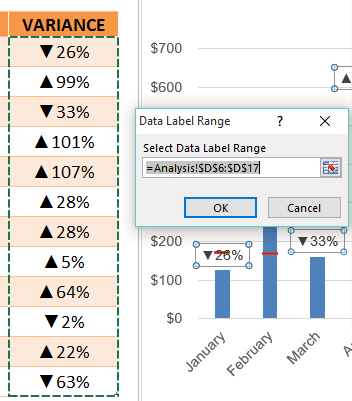
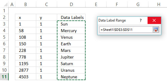
How-to Use Data Labels from a Range in an Excel Chart - Excel ...

Chart Data Labels in PowerPoint 2013 for Windows

How to Change Excel Chart Data Labels to Custom Values?

Share :